About Me
- Ravi Bhide
- Ravi is an armchair futurist and an aspiring mad scientist. His mission is to create simplicity out of complexity and order out of chaos.
Saturday, December 24, 2011
Stable Marriage Problem
Java-based implementation of the Gale-Shapley algorithm to solve the stable marriage problem can be found here: github/rbhide0/pudding.
Friday, December 16, 2011
Randomized two point sampling
While reading "Randomized Algorithms" by Motwani and Raghavan, I felt that the authors' treatment of the topic of "two point sampling" was a little too short and summarized. In this article, I provide some details around this topic.
Motivation
When using randomized algorithms, for a given input $x$, the usual strategy is to choose $n$ random numbers (a.k.a. "witnesses") and run a deterministic algorithm on the input using each of the random numbers. The intuition is that if the deterministic algorithm has a probability of error $\epsilon$ (e.g. $1/3$), $n$ independent runs reduce this probability to $\epsilon^n$ (e.g. $1/3^n$).
The above assumes that we have the option to choose $n$ independent random numbers. What happens if that option were constrained to choosing no more than a constant $c$ random numbers? We look at the simple case where we choose just 2 random numbers ($c=2$), giving it the name two-point. So, the main question we are trying to answer is the following:
The idea is to generate $n$ numbers based on the chosen 2 random numbers and use them in lieu of the $n$ purely independent random numbers. These generated numbers are dependent on the 2 chosen numbers. Hence they are not independent, but are pairwise independent. This loss of full independence reduces the accuracy of the algorithmic process, but it is still quite usable.
The Process
Motivation
When using randomized algorithms, for a given input $x$, the usual strategy is to choose $n$ random numbers (a.k.a. "witnesses") and run a deterministic algorithm on the input using each of the random numbers. The intuition is that if the deterministic algorithm has a probability of error $\epsilon$ (e.g. $1/3$), $n$ independent runs reduce this probability to $\epsilon^n$ (e.g. $1/3^n$).
The above assumes that we have the option to choose $n$ independent random numbers. What happens if that option were constrained to choosing no more than a constant $c$ random numbers? We look at the simple case where we choose just 2 random numbers ($c=2$), giving it the name two-point. So, the main question we are trying to answer is the following:
If our randomized algorithm reduced the probability of error to $\epsilon^n$ with $n$ random numbers, what can we expect about the probability of error with $2$ randoms? $\epsilon^2$ is an obvious bound, but can we do any better? It turns out that we can indeed do better and reduce the probability of error to $1/n$. This is significantly better than the constant, $\epsilon^2$.The High-level Idea
The idea is to generate $n$ numbers based on the chosen 2 random numbers and use them in lieu of the $n$ purely independent random numbers. These generated numbers are dependent on the 2 chosen numbers. Hence they are not independent, but are pairwise independent. This loss of full independence reduces the accuracy of the algorithmic process, but it is still quite usable.
The Process
- Choose a large prime number, $\rho$ (e.g. Mersenne prime, $2^{31}-1$).
- Define $\mathbb{Z}_\rho$ as the ring of integers modulo $\rho$. (e.g. $0,1,\cdots,2^{31}-2$)
- Choose 2 random numbers, $a$ and $b$ from $\mathbb{Z}_\rho$. (e.g. $a=2^{20}+781$ and $b=2^{27}-44$). These are the only independent random numbers that are picked for two-point sampling.
- Generate $n$ "pseudo-random" numbers $y_i=(a*i+b)\mod{\rho}$. E.g.
- $y_0=2^{27}-44$
- $y_1=(2^{20}+781)*1+2^{27}-44$
- $y_2=(2^{20}+781)*2+2^{27}-44$ and so on.
- Use each of $y_i$s as witnesses in lieu of independent random witnesses, for algorithm $\mathbi{A}$.
Notation
- Let $\mathbi{A}(x,y)$ denote the output of the execution of a deterministic algorithm $\mathbi{A}$ on input $x$ with witness $y$. We restrict this algorithm to return only $1$ or $0$. If the algorithm outputs $1$, we can be sure that $1$ is the right answer. If the algorithm outputs $0$, the right answer could be either $1$ or $0$.
- $\mathbi{A}(x,y)$ produces correct output (which could be either $1$ or $0$) with probability $p$, meaning it produces a possibly erroneous output (i.e. a $0$ instead of $1$) with probability $1-p$.
- Let $Y_i=\mathbi{A}(x,y_i)$ be a random variable, where $y_i$ is a psuedo-random number defined earlier. Note that the expected value of $Y_i$, $\mathbf{E}[Y_i]=p$, since $\mathbi{A}(x,y)$ produces a correct output with probability $p$.
- Let $Y=\sum{Y_i}$. By linearity of expectations, $\mathbf{E}[Y]=\mathbf{E}[\sum{Y_i}]=\sum{\mathbf{E}[Y_i]}=np$. Note that linearity of expectations is agnostic to the dependence between the random variables $Y_i$.
- Note that variance of $Y$, $\sigma^{2}_{Y}=np(1-p)$.
Derivation
We are trying to determine the error for the randomized process after $n$ runs of the deterministic algorithm $\mathbi{A}$. This is at most the probability of the event where each of the $n$ runs produced an erroneous output of $0$, i.e. each of $Y_i=0$, or equivalently, $Y=0$. (Note that some outputs of $0$ are not erroneous, hence the use of the words "at most".) So we are trying to determine $\mathbf{P}[Y=0]$.
Since $Y_i$s are not all independent, we cannot say:
\[\mathbf{P}[Y=0]=\prod{\mathbf{P}[Y_i=0]}\leq(1-p)^{n}\]
So, alternatively, we would like to know:
\[\mathbf{P}[|Y-\mathbf{E}[Y]|\geq\mathbf{E}[Y]]\]
which, by Chebyshev's inequality is:
\[\leq(\sigma_{Y}/\mathbf{E}[Y])^2\]
\[=\frac{np(1-p)}{n^2p^2}\]
\[=\frac{1-p}{np}\]
\[=O(\frac{1}{n})\]
Intuitively, this means that for any given error bound $\epsilon$, instead of requiring $O(\log(1/\epsilon))$ runs of the deterministic algorithm $\mathbi{A}$ in the case of $n$ independent random witnesses, we will require $O(1/\epsilon)$ runs in the case $2$ independent random witnesses. This is exponentially larger. So, it is not as efficient, but it is not the end of the world either!
In Closing
The above derivation shows that two random numbers are sufficient to minimize the error of a randomized algorithm below any given bound, although this comes with loss of some efficiency.
References
- Motwani, R. and Raghavan, P., Randomized Algorithms, 2007.
Friday, November 11, 2011
Greedy algorithm for grid navigation
For navigation problems that can be modeled as a grid with obstacles, we present a greedy algorithm that can determine a navigable path between any two given points on the grid.
Grid properties
Grid properties
- Rectangular board of size $m$ by $n$, so it has $m*n$ squares
- A square can be navigable or blocked (e.g. an obstacle)
- A square $(i, j)$ has the following adjacent squares:
- $(i-1, j-1)$ - corresponds to the south-west direction
- $(i-1, j)$ - corresponds to the west direction
- $(i-1, j+1)$ - corresponds to the north-west direction
- $(i, j-1)$ - corresponds to the south direction
- $(i, j+1)$ - corresponds to the north direction
- $(i+1, j-1)$ - corresponds to south-east direction
- $(i+1, j)$ - corresponds to the east direction and
- $(i+1, j+1)$ - corresponds to the north-east direction
- From a given square, one can navigate to any of the adjacent squares, unless that square is blocked or is beyond the board margins.
The objective
Given 2 points on the board - the source $s$ and the destination $d$, find a navigable path between $s$ and $d$.
Navigation algorithm
- We use a vector $\overrightarrow{v}$ ("the destination vector") to determine the direction of our destination from our current position $p$. \[\overrightarrow{v}=\overrightarrow{d}-\overrightarrow{p}=(d_x-p_x,d_y-p_y)\]
- A direction vector is a vector of unit length in a direction. E.g. east direction vector $\overrightarrow{i_{1}}=(1,0)$, north-east =$\overrightarrow{i_{2}}=(\frac{1}{\sqrt{2}},\frac{1}{\sqrt{2}})$.
- We use vector dot product to determine the degree of alignment between the destination vector $\overrightarrow{v}$ and each of the direction vectors ($\overrightarrow{i_{1}},\cdots,\overrightarrow{i_{8}}$).
- The direction vector with the best possible alignment with the destination vector, i.e. the one with the largest dot product, is the direction we take. In other words, the direction corresponding to the largest of {$(\overrightarrow{v}\cdot\overrightarrow{i_{1}}),(\overrightarrow{v}\cdot\overrightarrow{i_{2}}),\cdots,(\overrightarrow{v}\cdot\overrightarrow{i_{8}})$} is our choice.
- If we have already visited the square corresponding to this direction, we choose the next best direction available based on the dot product.
- We repeat the above steps till we reach our destination (or a pre-determined upper bound on the path length, at which point we abort.)
Properties of the algorithm
- This is a greedy algorithm. It chooses the direction to navigate in, based only on the current square it is in.
- For a grid with low obstacle ratio (e.g. less than half the squares are obstacles), this algorithm converges to a navigable path fairly quickly - in about 2 times the global shortest path or less, discounting outliers.
Implementation
You can find java source code here - https://github.com/briangu/amaitjo/blob/master/src/main/java/ravi/contest/ants/movement/NavigationAdvisor.java
You can find java source code here - https://github.com/briangu/amaitjo/blob/master/src/main/java/ravi/contest/ants/movement/NavigationAdvisor.java
Tuesday, November 8, 2011
Markov and Chebyshev inequalities
Markov inequality
Intuitively, this inequality states that the probability that a random variable's value is much greater than its mean is low and that the larger this value, the smaller its probability. It states that \[\mathbf{P}(X\geq a)\leq\frac{\mu}{a},\hspace{10 mm}\forall a>0\] where $\mu$ is the mean, a.k.a. the expected value $\mathbf{E}(X)$ of the random variable. Note that this inequality needs that the random variable $X$ take non-negative values.
Here are some examples
- $\mathbf{P}(X\geq 10)\leq\mu/10$, which doesn't say much since $\mu$ could be greater than $10$. But the next one is more interesting.
- $\mathbf{P}(X\geq10\mu)\leq1/10$, which means that the probability that a random variable is $10$ times its mean is less than or equal to $0.1$. Now that wasn't obvious before!
Chebyshev inequality
Unlike Markov inequality that involves just the mean, Chebyshev inequality involves the mean and the variance. Intuitively, it states that the probability of a random variable taking values far outside of its variance is low and the farther this value from its mean, the lower its probability. More formally, it states that \[\mathbf{P}(|X-\mu|\geq c)\leq\frac{\sigma^2}{c^2},\hspace{10 mm}\forall c>0\] This implies \[\mathbf{P}({X-\mu|\geq k\sigma)\leq\frac{1}{k^2}\] This means that the probability that a value falls beyond $k$ times the standard deviation is at most $1/k^2$. This inequality tends to give tighter bounds than Markov inequality.
More concretely
- $\mathbf{P}(|X-\mu|\geq2\sigma)\leq1/4$, which means that the probability that a random variable takes values outside of 2 times its standard deviation is less than $1/4$.
- $\mathbf{P}(|X-\mu|\geq3\sigma)\leq1/9$, which means that the probability that a random variable takes values outside of 3 times its standard deviation is less than $1/9$.
From Markov inequality to Chebyshev inequality
Derivation of Chebyshev inequality from Markov inequality is relatively straight forward. Let $Y=|X-\mu|^2$. According to Markov inequality \[\mathbf{P}(Y\geq c^2)\leq \mathbf{E}(Y)/c^2\] Since $\mathbf{E}(Y)=\sigma^2$ and $\mathbf{P}(Y\geq c^2)$ is equivalent to $\mathbf{P}(|X-\mu|\geq c)$, by substituting them, we get Chebyshev inequality \[\mathbf{P}(|X-\mu|\geq c)\leq\frac{\sigma^2}{c^2}\]
Sunday, August 14, 2011
Evaluating interviewers - Part 2
In this post, I show a method to mathematically evaluate an interviewer based on the job performance of the candidate that gets hired. This is a continuation of (but independent of) Evaluating Interviewers - Part 1, where I showed a method to evaluate an interviewer against other interviewers. I am replicating the definitions here from Part 1.
Definitions
What we expect from interview scores
We take the interviewer's score $s_{ij}$ as a prediction about the candidate $C_i$'s job performance once hired. The higher the score, the better the predicted job performance. E.g., when an interviewer gives a score of $3.1$ to candidate $C_1$ and $3.2$ to $C_2$, in effect, he is vouching for candidate $C_2$ to out-perform candidate $C_1$, by a margin proportional to $0.1$.
Secondly, we expect job performance to be directly and linearly proportional to the score. E.g., if scores of $3.1$ and $3.2$ translate to job performance ratings of $3.1$ and $3.2$ respectively, then a score of $3.3$ should translate to a job performance rating of $3.3$ or thereabouts.
In other words, we expect the following from our scores:

Good interviewer v/s Bad interviewer
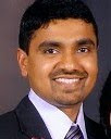
We classify an interviewer as good when there is high correlation between the score given by the interviewer to the candidate and the job performance of the candidate post-hire. The higher the correlation, i.e. the lower the variance, the better the interviewer. This is because a lower variance implies better predictability on part of the interviewer. Conversely, the higher the variance, the worse the interviewer.
Here is a graph of job performance (Y-axis) against interviewer score (X-axis) for a good interviewer:
Here is the graph for a bad interviewer. Notice the high variance, implying a low correlation between interview score and job performance:

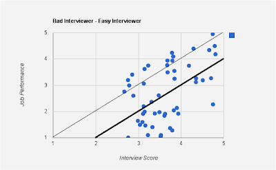
Easy v/s Hard interviewers
Variation from $y=x$ line doesn't necessarily indicate a bad interviewer. For an interviewer to be bad, the correlation between interview score and job performance should be low.
Here is an example of a good interviewer with high correlation between interview score and job performance, but whose mean is different from $y=x$ line.
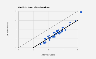

As opposed to the good interviewers, here are graphs for bad interviewers.
 In the above case, the interviewer is an easy interviewer - one who tends to give a higher scores than his peers, as seen from the mean line (thicker one parallel to $y=x$ line). However, the low correlation suggests that the interviewer's score does not accurately portray job performance.
Here is another bad interviewer - this time a hard one - one who tends to give lower scores than his peers.

Definitions
| Symbol | Definition |
| $C_i$ | $i^{th}$ candidate |
| $R_j$ | $j^{th}$ interviewer |
| $s_{ij}$ | score for the $i^{th}$ candidate by the $j^{th}$ interviewer (this is the grade, usually between 1 and 5, given by the interviewer to the candidate based on the interview) |
| $m_i$ | number of interviewers in the interview panel for candidate $i$ (the number of interviewers, usually between 4 and 8, that the candidate faces during the course of the interview process) |
| $n_j$ | number of candidates interviewed by interviewer $j$ (can be large, in tens or hundreds, especially for popular interviewers) |
| $\hat{n_j}$ | number of candidates interviewed by interviewer $j$ that joined the company/group |
| $p_i$ | job performance of $i^{th}$ candidate after joining the company/group (usually between 1 and 5, captured in a company-internal HRM system) |
| $s_i$ | average score given by the interview panel for the $i^{th}$ candidate, $s_i=\sum_{j}s_{ij}/{m_i}$ (usually between 1 and 5) |
What we expect from interview scores
We take the interviewer's score $s_{ij}$ as a prediction about the candidate $C_i$'s job performance once hired. The higher the score, the better the predicted job performance. E.g., when an interviewer gives a score of $3.1$ to candidate $C_1$ and $3.2$ to $C_2$, in effect, he is vouching for candidate $C_2$ to out-perform candidate $C_1$, by a margin proportional to $0.1$.
Secondly, we expect job performance to be directly and linearly proportional to the score. E.g., if scores of $3.1$ and $3.2$ translate to job performance ratings of $3.1$ and $3.2$ respectively, then a score of $3.3$ should translate to a job performance rating of $3.3$ or thereabouts.
In other words, we expect the following from our scores:
So we expect a plot of job performance (Y-axis) against interview score (X-axis) to be roughly linear for each interviewer, ideally along the $y=x$ line. We will discuss variations from this line and its implications later in the article.
- Ordinality: if $s_{aj}>s_{bj}$, then we hold interviewer $R_j$ to a prediction that candidate $C_a$ would outperform $C_b$ on the job.
- Linearity: job performance should be directly and linearly proportional to the score.

Good interviewer v/s Bad interviewer
We classify an interviewer as good when there is high correlation between the score given by the interviewer to the candidate and the job performance of the candidate post-hire. The higher the correlation, i.e. the lower the variance, the better the interviewer. This is because a lower variance implies better predictability on part of the interviewer. Conversely, the higher the variance, the worse the interviewer.
Here is a graph of job performance (Y-axis) against interviewer score (X-axis) for a good interviewer:
Here is the graph for a bad interviewer. Notice the high variance, implying a low correlation between interview score and job performance:

Easy v/s Hard interviewers
Variation from $y=x$ line doesn't necessarily indicate a bad interviewer. For an interviewer to be bad, the correlation between interview score and job performance should be low.
Here is an example of a good interviewer with high correlation between interview score and job performance, but whose mean is different from $y=x$ line.

Note that the above graph satisfies both the ordinality and linearity conditions and hence the interviewer is a good interviewer. The above graph is for an "easy" interviewer - one who tends to give a higher score than those of his peers. Notice that the mean line hangs below the $y=x$ line.
Here is another example of an interviewer with high correlation between interview score and job performance, but whose mean is different from $y=x$ line.
This is a "hard" interviewer - one who tends to give a lower score than those of his peers. Notice that the mean line hangs above the $y=x$ line.
As opposed to the good interviewers, here are graphs for bad interviewers.

Here is another bad interviewer - this time a hard one - one who tends to give lower scores than his peers.

The above graphs show that both easy and hard interviewers can be good interviewers. And on the flip side, both easy and hard interviewers can be bad interviewers. What really distinguishes good from bad is how "tightly" the points hug the mean line in the graph. With this as the background, here is some math that will order interviewers in the descending order of "goodness".
The Math
- Find the line parallel to $y=x$ that serves as the mean for all points in the graph. There can be different definitions for "mean" here - e.g. one that is a mean of all $x$ and $y$ co-ordinates of the points, one that minimizes the sum of distances to each point, etc. For simplicity, we choose the mean of all $x$ and $y$ coordinates for that interviewer, i.e. $\overline{x}_j$ and $\overline{y}_j$ for interviewer $R_j$ respectively.
\[\overline{x}_j=\frac{\sum_{k}s_{kj}}{\hat{n_j}}\]
\[\overline{y}_j}=\frac{\sum_{k}p_k}{\hat{n_j}}\]
So the dark line in the graph corresponds to $y=f_j(x)=x+(\overline{y}_j-\overline{x}_j)$.
- We compute the standard deviation of interviewer $R_j$'s score, $\sigma_j$, as follows.
\[\sigma_j=\sqrt{\frac{\sum_k{(p_{i_k}-f_j(s_{i_kj}))^2}}{\hat{n_j}-1}}\]
where subscript $i_k$ is used to indicate a candidate that the interviewer interviewed and was eventually hired. So, essentially, we are determining the variance of the points with respect to the line $y=f_j(x)$. The lower the $\sigma_j$, the better the interviewer is at predicting the job performance of the candidate.
- Alternatively, instead of the above steps, we can compute the correlation coefficient between the interview scores and the job performance score.
- Order interviewers $R_j$ based on descending order of $\sigma_j$ (or the correlation coefficient). This is the list of interviewers - from the best to the worst - in that order!
In Closing
- We outlined one approach to rank interviewers according to their ability to predict future performance of a job candidate.
- There are many ways in which the "goodness" of an interviewer can be defined. Each can alter our algorithm.
- There are many ways in which one can define average performance of the interviewer (the dark solid line in the graph). We choose a simple definition.
- Regardless of the customization applied to our algorithm, the graphs and the rankings can help the organization better the interview process, thus:
- if an interviewer is deemed "bad", retrain them
- if an interviewer is deemed "easy", perhaps discount their score for the candidate by their variance, $\sigma_j$ to determine what a regular interviewer's score would have been for that candidate.
- similarly, for a "hard" interviewer, add their variance $\sigma_j$ to normalize their score and bring it up to par with other "regular" interviewers.
Monday, August 1, 2011
Evaluating interviewers - Part 1
This post mathematically answers the question - "how to determine how good of an interviewer someone is".
Definitions
(Note: subscript $i$ is used for candidates and $j$ for interviewers)
Evaluating an interviewer w.r.t. other interviewers
Consider the random variable $X_j$ defined below, which is the difference between the score given by the $j^{th}$ interviewer and the average score given by the interview panel, for any candidate interviewed by $R_j$:
\[X_j=\{s_{ij}-s_i | R_j ~ \text{interviewed} ~ C_i\}\] We need to answer the following questions:
Categorization of interviewers
From the above answers regarding $X_j$, we can categorize interviewer $R_j$ into a few distinct types:
The "regular" interviewer

Most interviewers' distribution of $X_j$ would look like the above. (Perhaps not as sharp a drop off as shown above around 0 - I just couldn't draw a good graph!) This indicates that most interviewers' scores would be close to the average score given by the interview panel.
The "easy" interviewer

The easy interviewer tends to give, on an average, higher scores than the rest of the interview panel. This causes the bulk of the graph to shift beyond 0. The farther this hump from 0, the easier the interviewer. If you are an interviewee, this is the kind of interviewer you want!
The "hard-ass" interviewer

The hard interviewer tends to give lower scores than the rest of the interview panel. This causes hump of the graph to go below zero. The farther below zero, the harder the interviewer. If you are an interviewee, this is the kind of interviewer you want to avoid!
The "activist/extremist" interviewer

Some interviewers tend to artificially influence the outcome of the interview process by giving extreme scores - like "definitely hire" or "definitely no hire". The graph would not be as sharp as the one depicted above, but the idea is that there would be an above-average frequency of extreme values.

We evaluate interviewers in 2 complementary ways:
- With respect to other interviewers (covered in this blog post)
- With respect to interview candidate's actual job performance after being hired (covered in the next blog post).
Each method has its strengths. For example, we usually have a lot of data for method 1 (since there are more candidates interviewed than hired), making it easier to evaluate an interviewer relative to other interviewers. However, the true test of any interviewer is the consistency with which they can predict a candidate's job performance should they be hired. This data may be hard to come by (or integrate, with HRM systems). But each method can be used independently, or collectively.
(Note: subscript $i$ is used for candidates and $j$ for interviewers)
| Symbol | Definition |
| $C_i$ | $i^{th}$ candidate |
| $R_j$ | $j^{th}$ interviewer |
| $s_{ij}$ | score for the $i^{th}$ candidate by the $j^{th}$ interviewer (this is the grade, usually between 1 and 5, given by the interviewer to the candidate based on the interview) |
| $m_i$ | number of interviewers in the interview panel for candidate $i$ (the number of interviewers, usually between 4 and 8, that the candidate faces during the course of the interview process) |
| $n_j$ | number of candidates interviewed by interviewer $j$ (can be large, in tens or hundreds, especially for popular interviewers) |
| $\hat{n_j}$ | number of candidates interviewed by interviewer $j$ that joined the company/group |
| $p_i$ | job performance of $i^{th}$ candidate after joining the company/group (usually between 1 and 5, captured in a company-internal HRM system) |
| $s_i$ | average score given by the interview panel for the $i^{th}$ candidate, $s_i=\sum_{j}s_{ij}/{m_i}$ (usually between 1 and 5) |
Evaluating an interviewer w.r.t. other interviewers
Consider the random variable $X_j$ defined below, which is the difference between the score given by the $j^{th}$ interviewer and the average score given by the interview panel, for any candidate interviewed by $R_j$:
\[X_j=\{s_{ij}-s_i | R_j ~ \text{interviewed} ~ C_i\}\] We need to answer the following questions:
- What does a probability distribution of $X_j$ look like?
- What does the probability distribution of $X_j$ tell us about the interviewer $R_j$?
This is the random variable for the difference between the score given by an interviewer and the mean of the score received by the candidate. Clearly, expectation of $X$, $E(X)=0$. Moreover, we expect $X$ to have a normal distribution. So we expect some $X_j$ to be centered to the left of 0, some to the right of 0, but most others around 0.
So the answers to the above questions are:
- We expect the probability distribution of $X_j$ to be normal, centered around 0, on an average.
- $E(X_j)$ tells us about the type of interviewer $R_j$ is:
- $E(X_j)=0$ or more accurately, $|E(X_j)| < a\sigma$ (where $\sigma$ is the standard deviation of $X$, and $a>0$ is appropriately chosen) implies that the interviewer $R_j$ is a normal interviewer.
- $E(X_j)\geq a\sigma$ implies that interviewer $R_j$ generally gives higher scores than average.
- $E(X_j)\leq -a\sigma$ implies that interviewer $R_j$ generally gives lower scores than average.
Categorization of interviewers
From the above answers regarding $X_j$, we can categorize interviewer $R_j$ into a few distinct types:
The "regular" interviewer

Most interviewers' distribution of $X_j$ would look like the above. (Perhaps not as sharp a drop off as shown above around 0 - I just couldn't draw a good graph!) This indicates that most interviewers' scores would be close to the average score given by the interview panel.
The "easy" interviewer

The easy interviewer tends to give, on an average, higher scores than the rest of the interview panel. This causes the bulk of the graph to shift beyond 0. The farther this hump from 0, the easier the interviewer. If you are an interviewee, this is the kind of interviewer you want!
The "hard-ass" interviewer

The hard interviewer tends to give lower scores than the rest of the interview panel. This causes hump of the graph to go below zero. The farther below zero, the harder the interviewer. If you are an interviewee, this is the kind of interviewer you want to avoid!
The "activist/extremist" interviewer

Some interviewers tend to artificially influence the outcome of the interview process by giving extreme scores - like "definitely hire" or "definitely no hire". The graph would not be as sharp as the one depicted above, but the idea is that there would be an above-average frequency of extreme values.
The "clueless" interviewer

Some interviewers cannot correctly judge the potential of a candidate. Their scores would be all over the range, instead of a well-defined hump.
In closing
We presented a mathematical basis to compare interviewers. This yields a categorization of interviewers. In the next blog post, Evaluating Interviewers - Part II, we analyze how to evaluate an interviewer with respect to a hired candidate's job performance.
Sunday, July 10, 2011
Lebesgue Measure
Lebesgue measure is a measure of the length of a set of points, also called the $n$-dimensional "volume" of the set. So, intuitively:
The basics


- 1-dimensional volume is the length of a line segment,
- 2-dimensional volume is the area of a surface,
- 3-dimensional volume is the volume that we know of
- and so on.
The basics
- Lebesgue measure of a set of real numbers between $[a, b]$ is $b-a$. This is consistent with our intuitive understanding of the length of a line segment.
- Lebesgue measures are finitely additive. So the measure of a union of the set of points $[a, b]$ and $[c, d]$ is $(b-a) + (d-c)$. I.e. $\text{measure}([a,b]\bigcup[c,d])=(b-a)+(d-c)$. This is again consistent with our intuitive understanding of the sum of two line segments.
- In fact \[\text{measure}(\bigcup_{i=1}^{\infty} A_i)=\sum_{i=1}^{\infty}\text{measure}(A_i)\] The above applies to any $n$-dimensional measure (length, area, volume, etc.) This is consistent with our intuitive understanding of the sum of multiple line segments, areas, volumes, etc.
- countable sets (set of natural numbers, for example),
- uncountable sets (set of real numbers) and
- some seeming bizarre sets for which a Lebesgue measure cannot be defined.
Lebesgue measure for countable sets
- Lebesgue measure of integer points on the real line is $0$. This is because points are just locations on a real line and intuitively, integers are few and far between on a real line.
- Lebesgue measure of a countable set is $0$. This is a stronger statement than the above. It is interesting, since it implies that a set containing countably infinite number of points is also $0$. This is not surprising though, since between any two distinct integer points on the real line lie uncountably many real points. So intuitively, a countable set of points is just not large enough to have a non-zero Lebesgue measure!
- One implication of the above is that rational numbers have a measure of $0$. This is in spite of the fact that rationals are dense - i.e. between any 2 rational numbers, there are countably infinite number of rationals! So, countable infinity is no match for Lebesgue measure.
Lebesgue measure for uncountable sets
- As hinted earlier, Lebesgue measure for an uncountable number of contiguous points is non-zero. So for the set of points $[a, b]$, this is $b-a$.
- Removing a countable number of points from an uncountable set does not change its measure. E.g the measure of the half open set $(a, b]$ (which excludes just the point $a$) or the full open set $(a, b)$, which excludes both points $a$ and $b$ is $b-a$.
- One implication of the above is that if we were to remove, say, all rational numbers from the set $[a, b]$, its measure is still $b-a$. So we removed all countably infinite number of rationals, and yet the measure doesn't budge. Cool!
- Lebesgue measure of an uncountable set need not always be non-zero. Georg Cantor gave the construction of an uncountable set, called the Cantor set, which has uncountably infinite points, and yet has a measure of $0$, as shown in the next section.
Cantor Set - an uncountable set with 0 measure
- Start with the set of points $\mathbb{R}[0, 1]$.
- Divide it into 3 parts - $[0, 1/3]$, $(1/3, 2/3)$, $[2/3, 1]$ and remove the middle part $(1/3, 2/3)$ from the set, as depicted in the diagram below. (Note: the first line in the diagram represents $\mathbb{R}[0,1]$ and those below it represent the construction of the Cantor set as detailed in this and subsequent steps.)
- Of the remaining parts, divide each into 3 parts, as shown in the diagram above. E.g.
- Divide $[0, 1/3]$ into $[0, 1/9]$, $(1/9, 2/9)$, $[2/9, 1/3]$ and again remove the middle part $(1/9, 2/9)$ from the set.
- Similarly, divide $[2/3, 1]$ into $[2/3, 7/9]$, $(7/9, 8/9)$ and $[8/9, 1]$ and remove the middle part, $(7/9, 8/9)$ from the set.
- Keep repeating the above step, as shown in the diagram above.
- The segments that we end up removing have a combined measure of \[\frac{1}{3}+\frac{2}{9}+\frac{4}{27}+\frac{8}{81}\cdots=\frac{1}{3}\sum_{i=0}^{\infty}\bigg(\frac{2}{3}\bigg)^i=1\]
- This means that the number of points left has a Lebesgue measure of 0, even though the number of points left is uncountable!
- This is bizarre indeed. However, there is something even more bizarre. There are some sets that are not Lebesgue measurable! I.e. we cannot define a measure for them. A Vitali set is one such non-measurable set.
Vitali Set - a non-measurable set
Construction of this set relies on the Axiom of Choice and is slightly involved.
Construction of this set relies on the Axiom of Choice and is slightly involved.
- Definition: We define 2 points, $a$ and $b$, as equivalent if $a-b$ is a rational number. We denote this as $a\sim b$. Note that $a$ and $b$ themselves, don't have to be rationals for them to be equivalent. Examples of equivalence are:
- $\frac{1}{2}\sim \frac{1}{3}$, since $\frac{1}{2}-\frac{1}{3}=\frac{1}{6}$, a rational number.
- $\pi\sim\pi+\frac{1}{2}$, since $\pi-(\pi+\frac{1}{2})=-\frac{1}{2}$, a rational number.
- We partition the set of real numbers $\mathbb{R}[0, 1]$ into equivalence classes using the above definition. All points within an equivalence class are equivalent to each other, of course.

- Each equivalence class has countably many points, one corresponding to each rational number.
- There are uncountably many such equivalence classes, one corresponding to each irrational number (that is not separated from another irrational number by a rational distance).
- By axiom of choice, we can construct a set containing one point from each of these equivalence classes, which we call $V$, the Vitali set.
- Note that since elements of $V$ are drawn from $\mathbb{R}[0,1]$, $\text{measure}(V)\leq 1$.
- Definition: We define a translation of $V=\{v_0,v_1,v_2,\cdots\}$ called $V_q=\{v_0+q,v_1+q,v_2+q,\cdots\}$ where $q\in\mathbb{Q}[0,1]$, the set of rationals between $[0,1]$. So for each rational number $q$, we have a corresponding uncountable set $V_q$ as shown in the diagram above.
- Note that $\text{measure}(V)=\text{measure}(V_q)\quad\forall q\in\mathbb{Q}[0,1]$, since each $V_q$ is merely a translation of $V$.
- Also note that \[\bigcup_{q\in\mathbb{Q}[0,1]}V_q=\mathbb{R}[0,2]\] i.e. we just partitioned $\mathbb{R}[0,2]$ into countably many partitions, $V_q, q\in\mathbb{Q}[0,1]$, with each partition containing an uncountable number of points.
- With points (8) and (9) in mind, what is the Lebesgue measure of $V$?
- If it is $0$, from (8), it means that each of $V_q$ has a measure of $0$. It implies, from (9), that $\text{measure}(\mathbb{R}[0,2])=0$ which is false, since $\text{measure}(\mathbb{R}[0,2])=2$.
- If it is greater than $0$, say $a$, then from (8), each of $V_q$ has a measure of $a$. Hence, from (9), since there are infinitely many $q$s, $\text{measure}(\mathbb{R}[0,2])=\infty$ which is false, since $\text{measure}(\mathbb{R}[0,2])=2$.
- Hence, $V$ is not Lebesgue measurable!
In closing
We saw that there are some sets with Lebesgue measure $0$ and some with non-zero. We also saw that there are some uncountable sets with measure $0$ and some sets with an undefined measure.
References
We saw that there are some sets with Lebesgue measure $0$ and some with non-zero. We also saw that there are some uncountable sets with measure $0$ and some sets with an undefined measure.
References
- Wapner, Leonard, The Pea and the Sun, 2005.
- The Axiom of Choice (Wikipedia)
- Cantor Set (Wikipedia)
- Vitali Set (Wikipedia)
Saturday, July 2, 2011
Hyperwebster - an uncountable dictionary
Introduction
There are an infinite number of points on the real line. In fact, there are more points on any segment of the real line, no matter how small, than all of natural numbers combined. This was proved by Cantor using the diagonal argument.
To get an idea of the number of points on a real line, Dr. Ian Stewart gave the following construction of an infinite dictionary, the "hyperwebster".
Construction of the Hyperwebster
An enterprising publishing company decides to print a book containing all the words that can possibly created from the English alphabet A-Z. Since it is really a collection of letters of the alphabet in any order, of any length, we will see:
- some non-sensical words like "XWPBQI" and "NKPMZ",
- some real words like "SUN" and "MOON" and
- even some composite words like "SUNMOON" and "MOONSUN".
Since not all such words have meaning, the publishing company decides to include only the words in the book, without their associated meaning, if any.
So the "Hyperwebster" book looks like this:
A, AA, AAA, ..., AB, ABA, ABAA, ..., AC, ..., AZ, AZA, ...
B, BA, BAA, ..., BB, BBA, BBAA, ..., BC, ..., BZ, BZA, ...
C, CA, CAA, ..., CB, CBA, CBAA, ..., CC, ..., CZ, CZA, ...
Z, ZA, ZAA, ..., ZB, ZBA, ZBAA, ..., ZC, ..., ZZ, ZZA, ...
The staff at the publishing company realizes that it can partition the words into 26 volumes, one for each letter of the alphabet. So the Hyperwebster now looks like the following:
Volume B: B, BA, BAA, ..., BB, BBA, BBAA, ..., BC, ..., BZ, BZA, ...
Volume C: C, CA, CAA, ..., CB, CBA, CBAA, ..., CC, ..., CZ, CZA, ...
Volume Z: Z, ZA, ZAA, ..., ZB, ZBA, ZBAA, ..., ZC, ..., ZZ, ZZA, ...
Next, the staff realizes that all words in volume A start with the letter A, all words in volume B start with the letter B and so on. This means that the first letter in each word can be inferred from its volume and hence, the first letter can be dropped. Excellent! The publishing company just saved some ink by not printing an infinite number of letters.
The new volumes now look like this:
Volume A: A, AA, AAA, ..., B, BA, BAA, ..., C, ..., Z, ZA, ...
Volume B: A, AA, AAA, ..., B, BA, BAA, ..., C, ..., Z, ZA, ...
Volume C: A, AA, AAA, ..., B, BA, BAA, ..., C, ..., Z, ZA, ...
Volume Z: A, AA, AAA, ..., B, BA, BAA, ..., C, ..., Z, ZA, ...
The staff realizes that each volume now looks identical, except for the name of the volume. Why would anyone buy 26 identical copies of the same content? So, the decision is made to publish a single volume called "Hyperwebster", which looks like the following:
New hyperwebster:
A, AA, AAA, ..., B, BA, BAA, ..., C, ..., Z, ZA, ...
This turns out to be identical to the original hyperwebster that they started out with.
Original hyperwebster:
A, AA, AAA, ..., AB, ABA, ABAA, ..., AC, ..., AZ, AZA, ...
B, BA, BAA, ..., BB, BBA, BBAA, ..., BC, ..., BZ, BZA, ...
C, CA, CAA, ..., CB, CBA, CBAA, ..., CC, ..., CZ, CZA, ...
Z, ZA, ZAA, ..., ZB, ZBA, ZBAA, ..., ZC, ..., ZZ, ZZA, ...
The staff realizes that:
- the original volume can be partitioned into 26 different volumes,
- the first letter in each volume can be dropped, making each volume identical,
- and each volume now is really identical to the original volume
- and steps 1-3 can be applied ad infinitum.
The publishing company wisely abandons publishing the hyperwebster, even though each execution of steps 1-4 represent an infinite amount of savings!
Moral of the story
The content of the hyperwebster is equivalent to points on a real line (replace A-Z above with 0-9 and observe that it generates all real numbers). Any subset of the real line can be chopped up into infinitely many parts, each of which has the same number of points as the original. Each of the parts in turn can be chopped up into infinitely many subparts, each having the same number of points as the original, ad infinitum. Yeah, that's a lot of points! Continuum hypothesis states that the number of such points is aleph-1.
References
- Leonard M. Wapner, "The Pea and the Sun", 2005.
Wednesday, June 29, 2011
Continuum Hypothesis
This post looks at Cantor's continuum hypothesis and the relevant historical results around it.
Georg Cantor
Georg Cantor defined infinity in two steps. First he defined an infinite set and then "infinity":
Georg Cantor
Georg Cantor defined infinity in two steps. First he defined an infinite set and then "infinity":
- an infinite set is one that can be put in one-to-one correspondence with a proper subset of itself. E.g. natural numbers can be put in a one-to-one correspondence with the set of even numbers, which is a proper subset of the natural numbers. Here is the correspondence {0, 1, 2, 3, ... } maps to {0, 2, 4, 6, ...}.
- The cardinality of such a set is "infinity".
Cantor went a step ahead and defined a family of "infinities", each larger than the previous one.
- Cantor proved that even an infinite set cannot be put in one-to-one correspondence with its power set (i.e. the set of all its subsets), whose cardinality is 2^n (if the cardinality of the original set is n).
- This defines a family of "transfinite" cardinalities, each larger than the one before:
- aleph-0 (the cardinality of natural numbers),
- aleph-1 = 2^aleph-0,
- aleph-2 = 2^aleph-1
- and so on.
- Real numbers cannot be put in one-to-one correspondence with natural numbers. (See Cantor's diagonal argument). The cardinality of real numbers is called the cardinality of the continuum, c.
- Cantor hypothesized that c = aleph-1, which became known as the "Continuum Hypothesis". In other words, there is no transfinite cardinality between aleph-0 (cardinality of natural numbers) and c (cardinality of real numbers). But Cantor could not prove it. It turns out that there is a very good reason for that!
- By the way, Cantor called natural numbers or any subset thereof as countable, since they can be counted, i.e. put in one-to-one correspondence with 0, 1, 2, 3, ... . He called real numbers and higher transfinite cardinalities as uncountable, because they cannot be put in one-to-one correspondence with 0, 1, 2, 3, ... . (See Cantor's diagonal argument).
Kurt Godel
Kurt Godel came along and gave the world two "incompleteness" theorems.
- Informally, the first incompleteness theorem says that in any axiomatic system involving natural numbers, there are statements that cannot be proved or disproved within that system. In other words, there are some "undecidable" statements within the system.
- Stated differently, we can never come up with a finite set of axioms that can prove or disprove every statement in that system. Hence the system is always "incomplete".
- The intuition behind this is that there are only countably many provable statements, but uncountably many statements in the system. By the "pigeon hole" principle, some statements are unprovable. In fact, a vast majority of the statements are unprovable, since "uncountable" is much, much larger than "countable"!
- The second incompleteness theorem says that for some axiomatic systems, consistency cannot be proved within the system itself.
Axiom of Choice
- Simply stated, the axiom of choice says that given a bunch of non-empty sets, it is always possible to choose one element from each set to construct a new set.
- It seems logical and harmless. But complications arise when the original set has a large cardinality, e.g. aleph-1. How do we go about choosing one element from uncountably many sets? Where do we start - it cannot be put in one-to-one correspondence with natural numbers and hence cannot be labeled 1, 2, 3, ..., etc. So we wouldn't know which set is the first one, which is second and so on.
- One way to go about this complication is to just assume that there exists such a choice set and circumvent the above complexity.
- Not everyone agrees! So there are two different axiomatic set theories - one without the axiom of choice (ZF for Zermelo-Frankl, the formulators of set theory) and another with the axiom of choice (ZFC).
- Godel proved that the Axiom of Choice was consistent with ZF. In other words, ZFC is consistent.
The Finale
- Godel also proved that the continuum hypothesis was consistent with axiomatic set theory. In other words, it cannot be disproved within ZF.
- Paul Cohen comes along and proves that continuum hypothesis is independent of the other axioms in ZF. In other words, neither the continuum hypothesis nor its opposite can be proved within ZF. No wonder Cantor couldn't prove the "Continuum Hypothesis" from ZF axioms!
- Well, what does it all mean? Continuum hypothesis must either be true or be false, since aleph-1 must be either equal to c or not equal to c. The bottom line is that the result by Cohen and Godel say that neither the equality nor the inequality can be proved within the axiomatic system, no matter how smart you are or how hard you try!
- I, for one, believe that aleph-1 is indeed equal to c. In other words, there are no cardinalities in between that of the natural numbers and that of the real numbers.
References
- Leonard M. Wapner, "The Pea and the Sun", 2005.
Friday, May 27, 2011
Experiments in graph 3-coloring - block-cutpoint graph
Introduction
One way to reduce the runtime complexity of an algorithm is to partition the problem into smaller sub-problems, solve the sub-problems and combine these solutions to solve the original, bigger problem. This approach can be used when coloring a graph.
I investigated an approach that uses a block-cutpoint representation of the given graph. On a high level, here is the solution:
Definitions
Bi-connected graph
An undirected graph is bi-connected if any two vertices lie on a cycle. In other words, there are at least 2 distinct, disjoint paths between any two vertices. This concept is similar to that of a strongly connected component in a directed graph.
Block (aka Bi-connected component)
A bi-connected subgraph of a graph is called a block.
Cutpoint (aka cut vertex)
A vertex whose removal disconnects a graph is called a cut point or a cut vertex. Such vertices are "on the boundary" of a block. In Figure 1, they are shown in red color.

Block-Cutpoint graph

Coloring algorithm
Runtime complexity
Since the worst case running time is exponential in the number of nodes, say a^n for G, the runtime complexity of the above algorithm is a^n1 + a^n2 + ... + a^nm + O(n). This translates to O(a^max(n1, n2, ..., nm)) asymptotically.
In closing
This algorithm can be applied to n-coloring, not just 3-coloring. It reduces the time complexity if there are cut vertices in the graph. The more even the size of the blocks, the more the speed-up in run time.
One way to reduce the runtime complexity of an algorithm is to partition the problem into smaller sub-problems, solve the sub-problems and combine these solutions to solve the original, bigger problem. This approach can be used when coloring a graph.
I investigated an approach that uses a block-cutpoint representation of the given graph. On a high level, here is the solution:
- Given an undirected graph, construct its block-cutpoint graph.
- Solve the 3-coloring problem for each of the blocks.
- Combine the solution for each of the blocks to 3-color the original graph.
Definitions
Bi-connected graph
An undirected graph is bi-connected if any two vertices lie on a cycle. In other words, there are at least 2 distinct, disjoint paths between any two vertices. This concept is similar to that of a strongly connected component in a directed graph.
Block (aka Bi-connected component)
A bi-connected subgraph of a graph is called a block.
Cutpoint (aka cut vertex)
A vertex whose removal disconnects a graph is called a cut point or a cut vertex. Such vertices are "on the boundary" of a block. In Figure 1, they are shown in red color.

Block-Cutpoint graph
- A graph where a block is collapsed into a vertex,
- a cut vertex is represented as a vertex in this graph,
- there is an edge between a block vertex and a cut vertex only if the cut vertex is part of the block,
- there is an edge between two cut vertices only if there are adjacent in the original graph.

Interesting point to note is that any undirected graph can be represented as a tree of blocks and cutpoints, as shown in the figure above.
Coloring algorithm
- Partition given graph G into blocks B1, B2, ..., Bm.
- Color each of the blocks independently.
- The reconciliation step: two blocks, say B1 and B2, can share only 1 vertex (the cut vertex), say X.
- If X is colored with the same color, then we simply merge the colorings for B1 and B2.
- If X is colored differently in B1 and B2, say c1 and c2, respectively, then:
- we make X's color in B2 as c1 (its color in B1)
- All vertices in B2 colored as c2 are now colored as c1 and
- all vertices in B2 colored as c1 are now colored as c2.
- So in essence, we swapped colors c1 and c2 in B2.
- If we perform the reconciliation step in breadth first search order (BFS) of the block-cutpoint tree, we have a valid coloring for the original graph, provided each of the blocks has a valid coloring.
Runtime complexity
- Let the size of G be n.
- Let the sizes of the blocks B1, B2, ..., Bm be n1, n2, ..., nm, respectively.
Since the worst case running time is exponential in the number of nodes, say a^n for G, the runtime complexity of the above algorithm is a^n1 + a^n2 + ... + a^nm + O(n). This translates to O(a^max(n1, n2, ..., nm)) asymptotically.
In closing
This algorithm can be applied to n-coloring, not just 3-coloring. It reduces the time complexity if there are cut vertices in the graph. The more even the size of the blocks, the more the speed-up in run time.
Wednesday, May 18, 2011
Experiments in graph 3-coloring
3-coloring using independent sets
- By definition, vertices in an independent set (IS) share no edges. So these vertices can all be colored with one color.
- If after the removal of these vertices (and incident edges), the graph is 2-colorable, then we have a valid 3-coloring.
 |
| Fig 1: An independent set (red vertices) |
 |
| Fig 2: Graph without independent set |
 |
| Fig 3: Graph without independent set is 2-colorable |
 |
| Fig 4: Fully colored graph with 3 colors |
Interesting points about this approach
- Not all independent sets work, since G - IS may not be 2-colorable.
- Enumerating all independent sets is equivalent to enumerating the power set of the vertices and determining if they form an independent set. This has 2^v iterations, each taking about v^2 time. This is asymptotically better than 3^v iterations required for a brute force 3-coloring.
- If a graph is 3-colorable, then we can always find one color in a valid 3-coloring that is applied to at most floor(v/3) vertices. This implies that when enumerating all independent sets, we need to only find independent sets of size floor(v/3) or less. This is still O(2^n), by the way.
Optimization for this approach
- We start with brute force enumeration, as below, where 1 implies inclusion of the vertex and 0 its exclusion from the independent set.
- {1, 0, 0, ..., 0} - start by choosing v0
- {1, 1, 0, ...., 0} - after we choose v0 and v1 in the independent set.
- {1, 0, 1, ...., 0} - if we decide that v0 and v1 cannot be in an independent set (because they share an edge) and move on to v0 and v2.
- In general, if current selection is an independent set, keep the latest added vertex and include the next available vertex.
- In general, if current selection is not an independent set (because the latest vertex has one or more edges with previous vertices in the independent set), drop the latest added vertex and choose the next available one.
3-coloring with brute force
- This is exhaustive, brute force approach. We try each combination, till we find a valid coloring.
- Let the colors be 0, 1 and 2. Each color combination is an n-tuple. E.g. {0, 2, 1, 0, 0, 1, 1, 2, ...}. This colors vertex v0 with color 0, v1 with color 2, v2 with color 1 and so on.
- This is O(3^n), but seems to run faster in practice. Perhaps it has a tighter bound than O(3^n).
Optimization for this approach
- We order vertices arbitrarily as v0, v1, v2, ..., vn.
- We enumerate current color selection lexicographically. E.g.
- 0
- 0, 0, if the previous selection is a valid coloring
- 0, 0, 0 if the previous selection is a valid coloring
- 0, 0, 1 if the previous selection is not a valid coloring
- 0, 0, 2 if the previous selection is not a valid coloring
- 0, 1 if the previous selection is not a valid coloring
- 0, 1, 0 if the previous selection is a valid coloring
- and so on.
3-coloring greedily
- This is a simple approach, very fast in practice, but cannot color all colorable graphs.
- Order vertices by descending order of degree.
- Greedily choose the lowest color that is valid.
- Repeat above step till all vertices are colored.
- Runs in O(v^2) time.
Sunday, April 3, 2011
Flajolet-Martin algorithm
Flajolet-Martin algorithm approximates the number of unique objects in a stream or a database in one pass. If the stream contains $n$ elements with $m$ of them unique, this algorithm runs in $O(n)$ time and needs $O(log(m))$ memory. So the real innovation here is the memory usage, in that an exact, brute-force algorithm would need $O(m)$ memory (e.g. think "hash map").
As noted, this is an approximate algorithm. It gives an approximation for the number of unique objects, along with a standard deviation $\sigma$, which can then be used to determine bounds on the approximation with a desired maximum error $\epsilon$, if needed.
Given below are the following:
Intuition
If we had a good, random hash function that acted on strings and generated integers, what can we say about the generated integers? Since they are random themselves, we would expect:
The Flajolet-Martin algorithm
This is an informal description. Formal treatment can be found in the original paper listed in the reference section.
Java-based implementation
The code can be found here: FlajoletMartin.java. It uses lucene-core-3.0.3.jar or better.
As noted, this is an approximate algorithm. It gives an approximation for the number of unique objects, along with a standard deviation $\sigma$, which can then be used to determine bounds on the approximation with a desired maximum error $\epsilon$, if needed.
Given below are the following:
- intuition behind the algorithm
- the algorithm itself
- a java-based implementation
- some results using that implementation and
- some closing thoughts.
Intuition
If we had a good, random hash function that acted on strings and generated integers, what can we say about the generated integers? Since they are random themselves, we would expect:
- $1/2$ of them to have their binary representation end in $0$ (i.e. divisible by $2$),
- $1/4$ of them to have their binary representation end in $00$ (i.e. divisible by $4$)
- $1/8$ of them to have their binary representation end in $000$ (i.e. divisible by $8$)
- and in general, $1/2^n$ of them to have their binary representation end in $0^n$.
Turning the problem around, if the hash function generated an integer ending in $0^m$ bits (and it also generated integers ending in $0^{m-1}$ bits, $0^{m-2}$ bits, ..., $0^1$ bits), intuitively, the number of unique strings is around $2^m$.
To facilitate the above, this algorithm maintains 1 bit for each $0^i$ seen - i.e. 1 bit for 0, another for 00, another for 000, and so on. The output of the algorithm is based on the maximum of consecutive $0^i$ seen.
To facilitate the above, this algorithm maintains 1 bit for each $0^i$ seen - i.e. 1 bit for 0, another for 00, another for 000, and so on. The output of the algorithm is based on the maximum of consecutive $0^i$ seen.
The Flajolet-Martin algorithm
This is an informal description. Formal treatment can be found in the original paper listed in the reference section.
- Create a bit vector (bit array) of sufficient length $L$, such that $2^L>n$, the number of elements in the stream. Usually a 64-bit vector is sufficient since $2^{64}$ is quite large for most purposes.
- The i-th bit in this vector/array represents whether we have seen a hash function value whose binary representation ends in $0^i$. So initialize each bit to 0.
- Generate a good, random hash function that maps input (usually strings) to natural numbers.
- Read input. For each word, hash it and determine the number of trailing zeros. If the number of trailing zeros is k, set the k-th bit in the bit vector to 1.
- Once input is exhausted, get the index of the first 0 in the bit array (call this R). By the way, this is just the number of consecutive 1s (i.e. we have seen 0, 00, ...,
as the output of the hash function) plus one.
- Calculate the number of unique words as $2^R/\phi$, where $\phi$ is 0.77351. A proof for this can be found in the original paper listed in the reference section.
- The standard deviation of R is a constant: $\sigma(R)=1.12$. (In other words, R can be off by about 1 for 1-0.68=32% of the observations, off by 2 for about 1-0.95=5% of the observations, off by 3 for 1-0.997=0.3% of the observations using the Empirical rule of statistics). This implies that our count can be off by a factor of 2 for 32% of the observations, off by a factory of 4 for 5% of the observations, off by a factor of 8 for 0.3% of the observations and so on.
- (Averaging) Use multiple hash functions and use the average R instead.
- (Bucketing) Averages are susceptible to large fluctuations. So use multiple buckets of hash functions from the above step and use the median of the average R. This gives fairly good accuracy.
- Overall accuracy of this algorithm can be tuned by using appropriate number of hash functions in the averaging and bucketing steps. Of course, if more accuracy is desired, more hash functions need to be used, which implies higher computation cost.
Java-based implementation
The code can be found here: FlajoletMartin.java. It uses lucene-core-3.0.3.jar or better.
Results using the above implementation
- Wikipedia article on "United States Constitution" had 3978 unique words. When run ten times, Flajolet-Martin algorithm reported values of 4902, 4202, 4202, 4044, 4367, 3602, 4367, 4202, 4202 and 3891 for an average of 4198. As can be seen, the average is about right, but the deviation is between -400 to 1000.
- Wikipedia article on "George Washington" had 3252 unique words. When run ten times, the reported values were 4044, 3466, 3466, 3466, 3744, 3209, 3335, 3209, 3891 and 3088, for an average of 3492.
Closing thoughts
- The Flajolet-Martin algorithm approximates the number of unique elements quite well, using just O(log m) memory, where m is the number of unique words.
- During implementation, it was observed that this algorithm is quite sensitive to the hash function parameters. The hash functions suggested in the original paper ($h(x)=(M+N\sum{ord(x_j)*128^j)\mod(2^L)}$) work properly only when n is odd. Otherwise, the algorithm always reports the number of unique elements as 1 or 2! I chose both $M$ and $N$ as odd, as can be seen in the implementation.
References
- Flajolet, P. and Martin, N., Journal of Computer and System Sciences, 1985. PDF - http://citeseerx.ist.psu.edu/viewdoc/download?doi=10.1.1.81.3869&rep=rep1&type=pdf
- J. Ullman and A. Rajaraman, Mining of Massive Datasets, Chapter 3 - available at http://infolab.stanford.edu/~ullman/mmds/ch4.pdf
Wednesday, March 2, 2011
Locality Sensitive Hashing Explored
I was catching up on some new developments in the field of computer science in the past decade and came across Locality Sensitive Hashing (LSH) among other things. It piqued my interest, especially its theoretical aspect. Here I explore this topic informally.
Intuition
The idea is to have a hash function that is sensitive to distances. By that we mean that if two points are "close" to each other, the probability that this function hashes them to the same bucket is "high". Conversely, if the points are "far" apart, the probability that they get hashed to the same bucket is "low".
The beauty of such a function is that we can probabilistically determine if two points are "close enough" by hashing them, without determining their actual distance. This can be useful, especially when points are in high dimensions, their distance computation is complex or we just have too many points to work with. We sacrifice accuracy (since the computation is probabilistic) for speed (since the hash function is presumably computationally cheap). However, as indicated later, we can increase this accuracy arbitrarily by sacrificing some speed. :-)
Distance measure
Central to LSH is the concept of distance. In fact, it is the starting point for LSH. Here are some popular distance measures:
Hash function
Once a distance measure is decided upon, we need to come up with a locality sensitive hash function for that distance measure. Any random hash function may not necessarily work. In fact, it is not necessary that a distance measure will have an LSH at all! However, most well-known distance measures have known locality sensitive hash functions. E.g. Jaccard distance has "min-hash" functions that are locality sensitive.
More formally, a hash function f is said to be (d1, d2, p1, p2)-sensitive, if for any two points x and y:
Intuition
The idea is to have a hash function that is sensitive to distances. By that we mean that if two points are "close" to each other, the probability that this function hashes them to the same bucket is "high". Conversely, if the points are "far" apart, the probability that they get hashed to the same bucket is "low".
The beauty of such a function is that we can probabilistically determine if two points are "close enough" by hashing them, without determining their actual distance. This can be useful, especially when points are in high dimensions, their distance computation is complex or we just have too many points to work with. We sacrifice accuracy (since the computation is probabilistic) for speed (since the hash function is presumably computationally cheap). However, as indicated later, we can increase this accuracy arbitrarily by sacrificing some speed. :-)
Distance measure
Central to LSH is the concept of distance. In fact, it is the starting point for LSH. Here are some popular distance measures:
- Jaccard distance, if your points are sets
- edit distance, if your points are strings
- euclidean distance, if points are in n dimensions.
Regardless of which distance measure you choose for your purpose (you can invent one if you like), it must satisfy 3 conditions:
- d(x, x) = 0, i.e. distance between a point and itself is zero.
- d(x, y) = d(y, x), i.e. the distance measure is symmetric.
- d(x, y) + d(y, z) >= d(x, z) - known as the triangle inequality.
Hash function
Once a distance measure is decided upon, we need to come up with a locality sensitive hash function for that distance measure. Any random hash function may not necessarily work. In fact, it is not necessary that a distance measure will have an LSH at all! However, most well-known distance measures have known locality sensitive hash functions. E.g. Jaccard distance has "min-hash" functions that are locality sensitive.
More formally, a hash function f is said to be (d1, d2, p1, p2)-sensitive, if for any two points x and y:
- if d(x, y) < d1, then Probability(f(x) = f(y)) > p1, i.e. the probability that the two points get mapped by the hash function f to the same bucket is at least p1.
- and if d(x, y) > d2, then probability (f(x) = f(y)) < p2, i.e. the probability that the two points get mapped by the hash function f to the same bucket is at most p2.
There are some interesting observations here including that we only talk about d(x, y) being less than d1 or greater than d2, but nothing about when d1 < d(x, y) < d2, which as it turns out, is not important to the theory of LSH.
Family of hash functions
A locality sensitive hash function is useful in probabilistically determining if two points are "close" to each other or not. However, we are limited by the probabilities. E.g. a probability of p1 = 0.5 does not necessarily instill a reasonable confidence that the two points are close. However, if we have a family of such hash functions, then using probability theory, we can construct functions that give us arbitrarily high probabilities.
Here's how the construction goes:
- if f1, f2, ..., fn are (d1, d2, p1, p2)-sensitive, then we can AND them together to construct a (d1, d2, p1n, p2n)-sensitive hash function. This has the effect of reducing the probability.
- if f1, f2, ..., fn are (d1, d2, p1, p2)-sensitive, then we can OR them together to construct a (d1, d2, 1 - (1- p1)n, 1 - (1 - p2)n)-sensitive hash function. This has the effect of increasing the probability.
A combination of ANDs and ORs can get probabilities arbitrarily close to 1. The closer we want an LSH's p1 to 1 (and p2 to 0), the more ANDs and ORs we need to perform.
In closing
LSH is a cheap way to determine proximity of points in any space provided we can define a distance measure and come up with multiple hash functions that are locality sensitive. This technique has been applied to diverse problems like finding plagiarisms in student papers, detecting similar web pages, finger print matching, etc.
In my next post, I examine jaccard distance and min-hash function. Additionally, I look at other distance measures and some of their locality sensitive hashes.
References
- J. Ullman and A. Rajaraman, Mining of Massive Datasets, Chapter 3 - available at http://infolab.stanford.edu/~ullman/mmds/ch3.pdf
Subscribe to:
Posts (Atom)