Evaluating interviewers - Part 2

In this post, I show a method to mathematically evaluate an interviewer based on the job performance of the candidate that gets hired. This is a continuation of (but independent of) Evaluating Interviewers - Part 1, where I showed a method to evaluate an interviewer against other interviewers. I am replicating the definitions here from Part 1.

Definitions

Symbol	Definition
$C_i$	$i^{th}$ candidate
$R_j$	$j^{th}$ interviewer
$s_{ij}$	score for the $i^{th}$ candidate by the $j^{th}$ interviewer (this is the grade, usually between 1 and 5, given by the interviewer to the candidate based on the interview)
$m_i$	number of interviewers in the interview panel for candidate $i$ (the number of interviewers, usually between 4 and 8, that the candidate faces during the course of the interview process)
$n_j$	number of candidates interviewed by interviewer $j$ (can be large, in tens or hundreds, especially for popular interviewers)
$\hat{n_j}$	number of candidates interviewed by interviewer $j$ that joined the company/group
$p_i$	job performance of $i^{th}$ candidate after joining the company/group (usually between 1 and 5, captured in a company-internal HRM system)
$s_i$	average score given by the interview panel for the $i^{th}$ candidate, $s_i=\sum_{j}s_{ij}/{m_i}$ (usually between 1 and 5)

What we expect from interview scores
We take the interviewer's score $s_{ij}$ as a prediction about the candidate $C_i$'s job performance once hired. The higher the score, the better the predicted job performance. E.g., when an interviewer gives a score of $3.1$ to candidate $C_1$ and $3.2$ to $C_2$, in effect, he is vouching for candidate $C_2$ to out-perform candidate $C_1$, by a margin proportional to $0.1$.

Secondly, we expect job performance to be directly and linearly proportional to the score. E.g., if scores of $3.1$ and $3.2$ translate to job performance ratings of $3.1$ and $3.2$ respectively, then a score of $3.3$ should translate to a job performance rating of $3.3$ or thereabouts.

In other words, we expect the following from our scores:

1. Ordinality: if $s_{aj}>s_{bj}$, then we hold interviewer $R_j$ to a prediction that candidate $C_a$ would outperform $C_b$ on the job.
2. Linearity: job performance should be directly and linearly proportional to the score.

So we expect a plot of job performance (Y-axis) against interview score (X-axis) to be roughly linear for each interviewer, ideally along the $y=x$ line. We will discuss variations from this line and its implications later in the article.

Good interviewer v/s Bad interviewer

We classify an interviewer as good when there is high correlation between the score given by the interviewer to the candidate and the job performance of the candidate post-hire. The higher the correlation, i.e. the lower the variance, the better the interviewer. This is because a lower variance implies better predictability on part of the interviewer. Conversely, the higher the variance, the worse the interviewer.

Here is a graph of job performance (Y-axis) against interviewer score (X-axis) for a good interviewer:

Here is the graph for a bad interviewer. Notice the high variance, implying a low correlation between interview score and job performance:

Easy v/s Hard interviewers
Variation from $y=x$ line doesn't necessarily indicate a bad interviewer. For an interviewer to be bad, the correlation between interview score and job performance should be low.

Here is an example of a good interviewer with high correlation between interview score and job performance, but whose mean is different from $y=x$ line.

Note that the above graph satisfies both the ordinality and linearity conditions and hence the interviewer is a good interviewer. The above graph is for an "easy" interviewer - one who tends to give a higher score than those of his peers. Notice that the mean line hangs below the $y=x$ line.

Here is another example of an interviewer with high correlation between interview score and job performance, but whose mean is different from $y=x$ line.

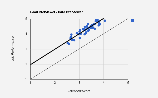
This is a "hard" interviewer - one who tends to give a lower score than those of his peers. Notice that the mean line hangs above the $y=x$ line.

As opposed to the good interviewers, here are graphs for bad interviewers.

In the above case, the interviewer is an easy interviewer - one who tends to give a higher scores than his peers, as seen from the mean line (thicker one parallel to $y=x$ line). However, the low correlation suggests that the interviewer's score does not accurately portray job performance.

Here is another bad interviewer - this time a hard one - one who tends to give lower scores than his peers.

The above graphs show that both easy and hard interviewers can be good interviewers. And on the flip side, both easy and hard interviewers can be bad interviewers. What really distinguishes good from bad is how "tightly" the points hug the mean line in the graph. With this as the background, here is some math that will order interviewers in the descending order of "goodness".

The Math

1. Find the line parallel to $y=x$ that serves as the mean for all points in the graph. There can be different definitions for "mean" here - e.g. one that is a mean of all $x$ and $y$ co-ordinates of the points, one that minimizes the sum of distances to each point, etc. For simplicity, we choose the mean of all $x$ and $y$ coordinates for that interviewer, i.e. $\overline{x}_j$ and $\overline{y}_j$ for interviewer $R_j$ respectively.

\[\overline{x}_j=\frac{\sum_{k}s_{kj}}{\hat{n_j}}\]

\[\overline{y}_j}=\frac{\sum_{k}p_k}{\hat{n_j}}\]

So the dark line in the graph corresponds to $y=f_j(x)=x+(\overline{y}_j-\overline{x}_j)$.

2. We compute the standard deviation of interviewer $R_j$'s score, $\sigma_j$, as follows.

\[\sigma_j=\sqrt{\frac{\sum_k{(p_{i_k}-f_j(s_{i_kj}))^2}}{\hat{n_j}-1}}\]

where subscript $i_k$ is used to indicate a candidate that the interviewer interviewed and was eventually hired. So, essentially, we are determining the variance of the points with respect to the line $y=f_j(x)$. The lower the $\sigma_j$, the better the interviewer is at predicting the job performance of the candidate.

3. Alternatively, instead of the above steps, we can compute the correlation coefficient between the interview scores and the job performance score.
4. Order interviewers $R_j$ based on descending order of $\sigma_j$ (or the correlation coefficient). This is the list of interviewers - from the best to the worst - in that order!

In Closing

• We outlined one approach to rank interviewers according to their ability to predict future performance of a job candidate.
• There are many ways in which the "goodness" of an interviewer can be defined. Each can alter our algorithm.
• There are many ways in which one can define average performance of the interviewer (the dark solid line in the graph). We choose a simple definition.
• Regardless of the customization applied to our algorithm, the graphs and the rankings can help the organization better the interview process, thus:

1. if an interviewer is deemed "bad", retrain them
2. if an interviewer is deemed "easy", perhaps discount their score for the candidate by their variance, $\sigma_j$ to determine what a regular interviewer's score would have been for that candidate.
3. similarly, for a "hard" interviewer, add their variance $\sigma_j$ to normalize their score and bring it up to par with other "regular" interviewers.